
Step 3: Calculating Population Growth Rate (PGR)
This section focuses on preparing population grid data to derive population statistics for different time periods within your urban areas.
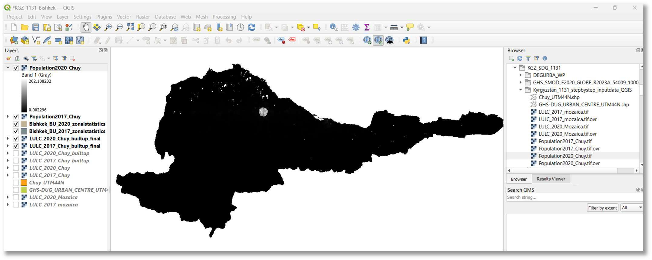
15. Add WorldPop raster datasets to map: Add the WorldPop raster datasets for 2017 and 2020 to your QGIS map canvas (e.g., drag-and-drop Population2017_Chuy.tif and Population2020_Chuy.tif).
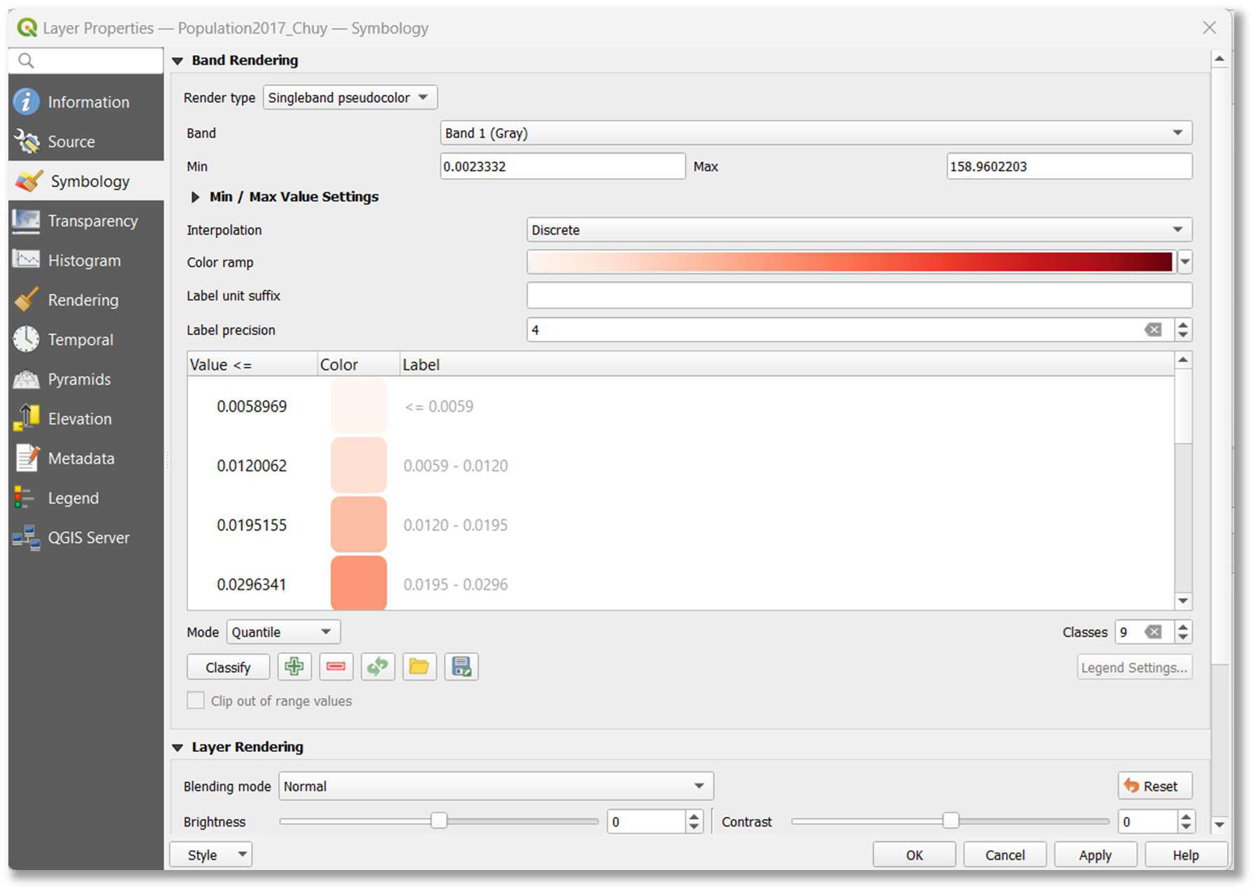
16. Enhance population grid visualization (symbology): To better understand the population distribution within the grids, change the symbology for both raster layers.
- Right-click each population layer in the ‘Layers’ panel and select Properties > Symbology.
- Set ‘Render type’ to ‘Singleband pseudocolor’.
- Under ‘Min / Max Value Settings’, choose an appropriate ‘Interpolation’ (e.g., ‘Discrete’ or ‘Linear’) and ‘Color ramp’ (e.g., ‘Reds’ for population density).
- Adjust ‘Mode’ (e.g., ‘Quantile’ or ‘Equal Interval’) and ‘Classes’ to define visual ranges.
- Click ‘Apply’ then ‘OK’.
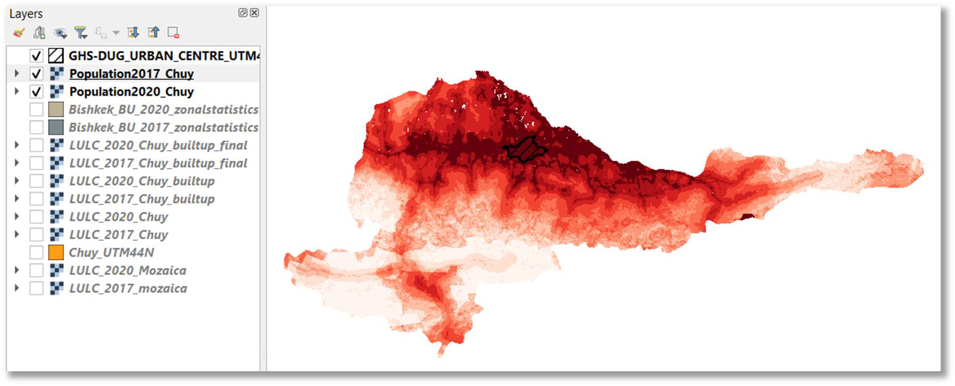
The image below shows the visualized population grid:
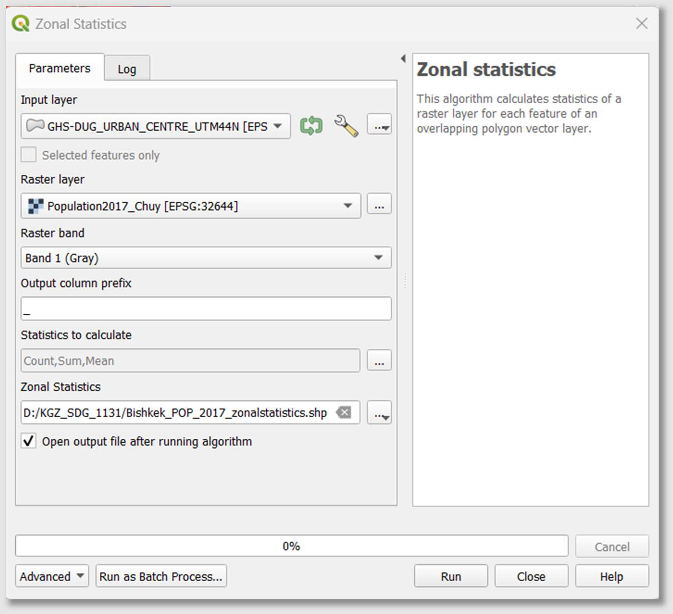
17. Calculate population statistics for 2017 and 2020 within urban boundaries: Run the Zonal statistics tool for both Population2017_Chuy.tif and Population2020_Chuy.tif rasters. This will sum the population values within your DEGURBA urban areas for each year.
- In the ‘Processing Toolbox’, search for “Zonal Statistics” and choose Raster analysis > Zonal Statistics.
- For 2017:
- Set ‘Input layer’ to your DEGURBA urban area shapefile (e.g., GHS-DUG_URBAN_CENTRE_UTM44N).
- Set ‘Raster layer’ to Population2017_Chuy.tif.
- Under ‘Statistics to calculate’, ensure ‘Sum’ is selected.
- Specify the output shapefile as D:/SDG_1131_Project/Bishkek_POP_2017_zonalstatistics.shp.
- Click ‘Run’.
- For 2020:
- Repeat the process with ‘Raster layer’ set to Population2020_Chuy.tif.
- Specify the output shapefile as D:/SDG_1131_Project/Bishkek_POP_2020_zonalstatistics.shp.
- Click ‘Run’.
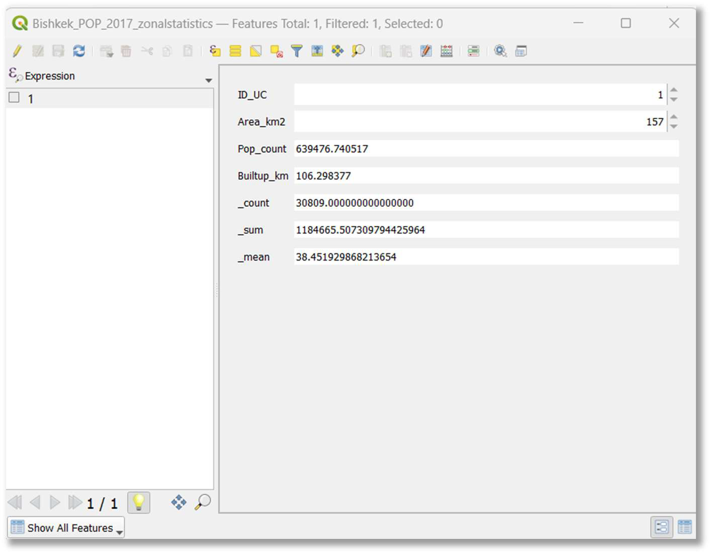
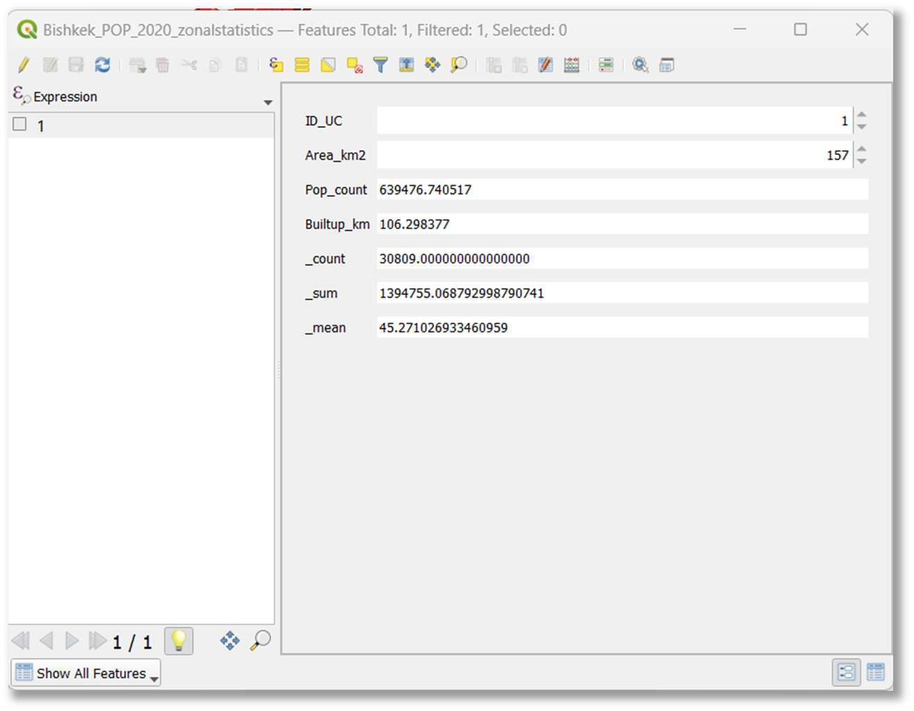
18. Review population statistics for 2017 and 2020: Open the attribute tables for the layers Bishkek_POP_2017_zonalstatistics and Bishkek_POP_2020_zonalstatistics to obtain the total population values for Bishkek in 2017 and 2020, respectively.
- For 2017, the example shows a sum of 1184665.50…, which translates to approximately 1,184,665 inhabitants.
- For 2020, the example shows a sum of 1394755.06…, which translates to approximately 1,394,755 inhabitants.
NOTE: Creating a population spatial grid based on national census data and adopting this methodology can result in advanced spatial insights and further in-depth analysis related to land consumption and population dynamics in urban areas.