Estimating the model

7 Estimating the model

In this section, we will estimate the model we have been building up to. We will use an updated version of the povmap package, which is not yet on CRAN, so we will download the GitHub version.

7.1 povmap

The povmap package contains many functions that enable small area estimation using a variety of methods. The package is under active development, but its CRAN version is stable. You can find a pdf of the package’s documentation here and you can find more updated versions – that are not yet on CRAN – on the World Bank’s Sub-Saharan Africa Statistical Team’s GitHub page here. As noted, we are not going to use the CRAN version. Instead, we are going to use a more updated version that includes different options for the ebp() function. Here is the code to install the package off GitHub:

devtools::install_github("SSA-Statistical-Team-Projects/povmap", ref = "david3")

If you receive an error trying to install povmap – for example, if the authors of that package update the CRAN version and remove the david3 branch – we have also uploaded a .zip file of the package on our GitHub page. You can download the compressed .zip file and then install it using devtools::install_local(PATH), where PATH is the path to the .zip file.

For this example, we will be using the function ebp(), which stands for empirical best prediction (Molina and Rao, 2010). We will be estimating a sub-area model, in which the admin4 geography is the sub-area, and predicting at the admin3 (TA – or Traditional Authority – in Malawi) level.

In the previous section, we already set up our data for the estimation. Our outcome variable is contained in the pov object and our predictors are in the ‘features’ object.

The simplest specification of our model is as follows:

results <- ebp(
1  fixed = ebpformula,
2  pop_data = features,
3  pop_domains = "TA_CODE",
4  smp_data = pov,
5  smp_domains = "TA_CODE",
6  MSE = TRUE,
7  transformation = "arcsin",
8  na.rm = TRUE
  )

1

fixed = ebpformula: This is the formula we created above, which includes the non-zero coefficients selected using lasso.

2

pop_data = features: This is the dataset that includes the predictors for the population. In this case, it is the features object.

3

pop_domains = "TA_CODE": This is the identifier for the area in the population data. In our example, it is the admin3 identifier, the TA_CODE.

4

smp_data = pov: This is the dataset that includes the outcome of interest. This is created from a survey, so it does not cover all of the admin3 areas. In our example, it is the pov object.

5

smp_domains = "TA_CODE": This is the identifier for the area in the sample data. It has the same name as the pop_domains in this case.

6

MSE = TRUE: This tells the function to calculate variance estimates.¹

7

transformation = "arcsin": This is the transformation we used above. Note that the default for ebp() is a box-cox transformation. If you do not want to use a transformation, you can specify transformation = "no". Importantly, we need to give ebp() the untransformed outcome variable in the pov object, since we are asking ebp90 to then make the transformation.

8

na.rm = TRUE: This tells the function to remove missing values. This is important because the function will not run if there are any missing values. Ideally, you should clean your data such that this option is not strictly necessary (i.e. there will already be no missing values).

7.2 Specifying options e.g. weighting, transformations, benchmarking

We have already seen the use of one option: the transformation. But ebp() also takes other options, as well. Specifically, let’s discuss weights and benchmarking options.

For weights, we can specify two different types of weights: sample weights and population weights.

• Sample weights are weights that are used to adjust for the fact that some observations are more likely to be in the sample than others. In our case, we have already created these weights in the pov object; they are in the column called total_weights.

• Population weights are used to adjust for the fact that different subareas have different populations. Since we want to calculate a population-weighted poverty rate at the admin3 level, we can use the pop_weights option. We have estimated population (from WorldPop) in the column entitled mwpop in the features data.

We can also benchmark the estimates such that they match existing official statistics for higher level geographies. In our example, we have data only from the Northern region of Malawi. The 2020 Malawi Poverty Report states that the official poverty rate for the region is 32.9 percent. We are using proportions, so we want to benchmark the overall values to equal 0.329, on average. We need to give the ebp function a named vector, where the name equals the indicator we want to benchmark and the value is the benchmark value. The function can benchmark for the the "Mean" or "Head_Count". Although we are estimating head count poverty, we are actually estimating the mean poverty rate in each admin3 area. We can create the named vector as follows:

bench <- c("Mean" = 0.329)

Putting this all together, we can estimate our final model:

results <- ebp(
  fixed = ebpformula,
  pop_data = features,
  pop_domains = "TA_CODE",
  smp_data = pov,
  smp_domains = "TA_CODE",
  MSE = TRUE,
  transformation = "arcsin",
  na.rm = TRUE,
1  weights = "total_weights",
2  pop_weights = "mwpop",
3  weights_type = "nlme",
4  benchmark = bench
  )

1

weights = "total_weights": This is the sample weight. It is used to adjust for the fact that the survey data is not a simple random sample.

2

pop_weights = "mwpop": This is the population weight. It is used to adjust for the fact that different subareas have different populations.

3

weights_type = "nlme": This option is required when using an arcsin transformation. The default weighting type does not work with the arcsin transformation, unfortunately.

4

benchmark = bench: This is the benchmarking option. We are benchmarking the mean poverty rate to equal 0.329, on average.

7.3 Verifying the assumptions

Now that we have estimated the model, we can look at some statistics to verify the assumptions of the model. Since we use a parametric bootstrap, the assumption of normality is important for both the residuals and the random effects. We can look at statistics for normality using the summary() function:

summary(results)

Empirical Best Prediction

Call:
 ebp(fixed = poor ~ average_masked + barecoverfraction + urbancoverfraction + 
    mosaik1 + mosaik39 + mosaik156 + mosaik268 + mosaik396 + 
    mosaik459 + mosaik464, pop_data = features, pop_domains = "TA_CODE", 
    smp_data = pov, smp_domains = "TA_CODE", transformation = "arcsin", 
    MSE = TRUE, na.rm = TRUE, weights = "total_weights", pop_weights = "mwpop", 
    weights_type = "nlme", benchmark = bench)

Out-of-sample domains:  27 
In-sample domains:  49 
Out-of-sample subdomains:  0 
In-sample subdomains:  0 

Sample sizes:
Units in sample:  107 
Units in population:  2908 
                   Min. 1st Qu. Median      Mean 3rd Qu. Max.
Sample_domains        1     1.0      2  2.183673       3    7
Population_domains    1     5.5     18 38.263158      44  300

Explanatory measures for the mixed model:
 Marginal_R2 Conditional_R2 Marginal_Area_R2 Conditional_Area_R2
   0.3064676       0.363829        0.6806806           0.7700488

Residual diagnostics for the mixed model:
                Skewness Kurtosis Shapiro_W  Shapiro_p
Error         -0.1317611 3.652988 0.9909934 0.70316526
Random_effect  0.3867831 5.282390 0.9465488 0.02682613

Estimated variance of random effects:
                 Variance
Error         0.030851330
Random_effect 0.002781762

ICC:  0.08270908 

Shrinkage factors 
        gamma.Min. gamma.1st.Qu. gamma.Median gamma.Mean gamma.3rd.Qu.
TA_CODE 0.08270908    0.08270908    0.1416945  0.1477909      0.189778
        gamma.Max.
TA_CODE   0.378302

Transformation:
 Transformation Shift_parameter
         arcsin               0

Specifically, there is a section of the output entitled “Residual diagnostics for the mixed model.” Here, we can see the skewness and the kurtosis. For a normal distribution, these should be equal to zero and three, respectively. In this case, the kurtosis is a bit high for both the residuals and the random effects. This is not ideal, but given their values it is also not a huge cause for concern. We can also plot them using plot(results):²

plot(results)

7.4 Evaluating results

The final step is to evaluate the results. We can do this in a number of ways. First, we can look at the r-squared value. Second, we can look at the change in precision from the sample to the modeled estimates. Third, we can validate the accuracy of the estimates. We will discuss each of these in turn.

7.4.1 R-squared

The summary() function above also output information about r-squared. There are four separate r-squared values: the marginal area r-squared, the marginal unit r-squared, the conditional area r-squared, and the conditional unit r-squared. From experience, it is the area r-squared values that are most relevant to the quality of the output. This explains the proportion of the variance across areas that is explained by the model (either the coefficients or both the coefficients and the random effects). In our example, the conditional area r-squared is approximately 0.77, which is relatively high.

7.4.2 How much does precision change?

Let’s compare the new estimates to sample estimates. First, let’s extract the results from the results object. Here, we are going to extract three things: the admin3 idenfitier, the modeled poverty rate, and the modeled variance estimates:

1resultsebp <- as_tibble(cbind(TA_CODE = levels(results$ind$Domain),
2  poor_ebp = results$ind$Mean_bench,
3  poor_ebp_var = results$MSE$Mean_bench))

1

TA_CODE = levels(results$ind$Domain): This is the admin3 identifier. It is stored as a factor variable, so we extract the levels instead of the values.

2

poor_ebp = results$ind$Mean: This is the modeled poverty rate after benchmarking. It is stored in the ind object, which is the modeled estimates. Note that the ind object also includes the unbenchmarked estimates (in the column Mean).

3

poor_ebp_var = results$MSE$Mean_bench: This is the modeled variance estimate. It is stored in the MSE object, which is the modeled variance estimates. The same note about benchmarking applies here.

Next, we will estimate sample estimates. We can do this using the direct() function from the povmap package. We are going to use the household-level data for this, not the admin4 data. The raw survey data is saved as a Stata file, so we read it using the read_dta() function from the haven package.³

hhs <- read_dta("data/ihshousehold/ihs5_consumption_aggregate.dta")
hhs$weights <- hhs$adulteq*hhs$hh_wgt
estimates <- direct(
  y = "poor",
  smp_data = hhs,
  smp_domains = "TA",
  weights = "weights",
  var = TRUE,
  HT = TRUE
  )
resultsdirect <- as_tibble(cbind(TA_CODE = levels(estimates$ind$Domain),
  poor_dir = estimates$ind$Mean,
  poor_dir_var = estimates$MSE$Mean))

Now let’s join the two together and turn the values into numeric values, as well as take the square root of the variance estimates to turn them into standard errors:

resultsall <- resultsebp |>
  left_join(resultsdirect, by = "TA_CODE")
resultsall <- resultsall |>
  mutate(poor_ebp = as.numeric(poor_ebp),
    poor_ebp_var = sqrt(as.numeric(poor_ebp_var)),
    poor_dir = as.numeric(poor_dir),
    poor_dir_var = sqrt(as.numeric(poor_dir_var)))
saveRDS(resultsall, "assets/resultsall.rds")

Here are the results:

Table 1: Comparison of in-sample and out-of-sample estimates

	Direct		EBP
	Rate	SE	Rate	SE
In sample	0.318	0.128	0.306	0.070
Out of sample	NA	NA	0.231	0.114

The mean poverty rates are quite similar, but note that the standard errors are much smaller for the modeled estimates. This is because the model is able to “borrow strength” from other areas. In this example, the mean standard error decreases by about 45 percent, which is equivalent to a gain in precision from increasing the size of the survey by a factor of approximately 3.3.

7.4.3 How can we validate the accuracy?

Validating the accuracy of results can be difficult. When developing new methods, we often use census data to provide “ground truth” information, which we can compare with our modeled estimates. Of course, if we always had access to census estimates of poverty, we would not need to estimate the small area model in the first place.

In our case, with a sample, we can use the sample data itself to validate accuracy. How? Through cross validation. We can estimate the model on a subset of the data and then predict on the remaining data, similar to what we did above with lasso to select the variables. Here is a very simple example, where we only estimate poverty for one “fold,” or one-fifth of the data. Importantly, however, we are estimating poverty at the admin3 (TA) level, which means we need to assign admin4 (EA) to folds at the admin3 level.

# get TAs
povTAs <- unique(pov$TA_CODE)
# assign folds - set seed so we get consistent results
set.seed(2025)
povTAs <- cbind(TA_CODE = povTAs, foldTA = sample(1:5, length(povTAs), replace = TRUE))
# add back to pov
pov <- pov |>
  left_join(as_tibble(povTAs), by = "TA_CODE")

resultscv <- ebp(
  fixed = ebpformula,
  pop_data = features,
  pop_domains = "TA_CODE",
  smp_data = pov[pov$foldTA!=1,],
  smp_domains = "TA_CODE",
  MSE = TRUE,
  transformation = "arcsin",
  na.rm = TRUE,
  weights = "total_weights",
  pop_weights = "mwpop",
  weights_type = "nlme",
  benchmark = bench
  )
povfold1 <- pov |>
  filter(foldTA==1) |>
  group_by(TA_CODE) |>
  summarise(poor = weighted.mean(poor, total_weights, na.rm = TRUE)) |>
  ungroup()
resultscv <- as_tibble(cbind(TA_CODE = levels(resultscv$ind$Domain),
  poor_ebp = resultscv$ind$Mean_bench,
  poor_ebp_var = resultscv$MSE$Mean_bench))
# turn to numeric in order to join with povfold1
resultscv$TA_CODE <- as.numeric(resultscv$TA_CODE)
resultscv <- povfold1 |>
  left_join(resultscv, by = "TA_CODE") |>
  mutate(poor_ebp = as.numeric(poor_ebp),
    poor_ebp_var = sqrt(as.numeric(poor_ebp_var)))
resultscv

Now, we can look at statistics like correlations between the modeled and sample estimates, as well as the mean squared error. We can also plot the results, as in Figure 1.

Figure 1: Predicted-true poverty rates

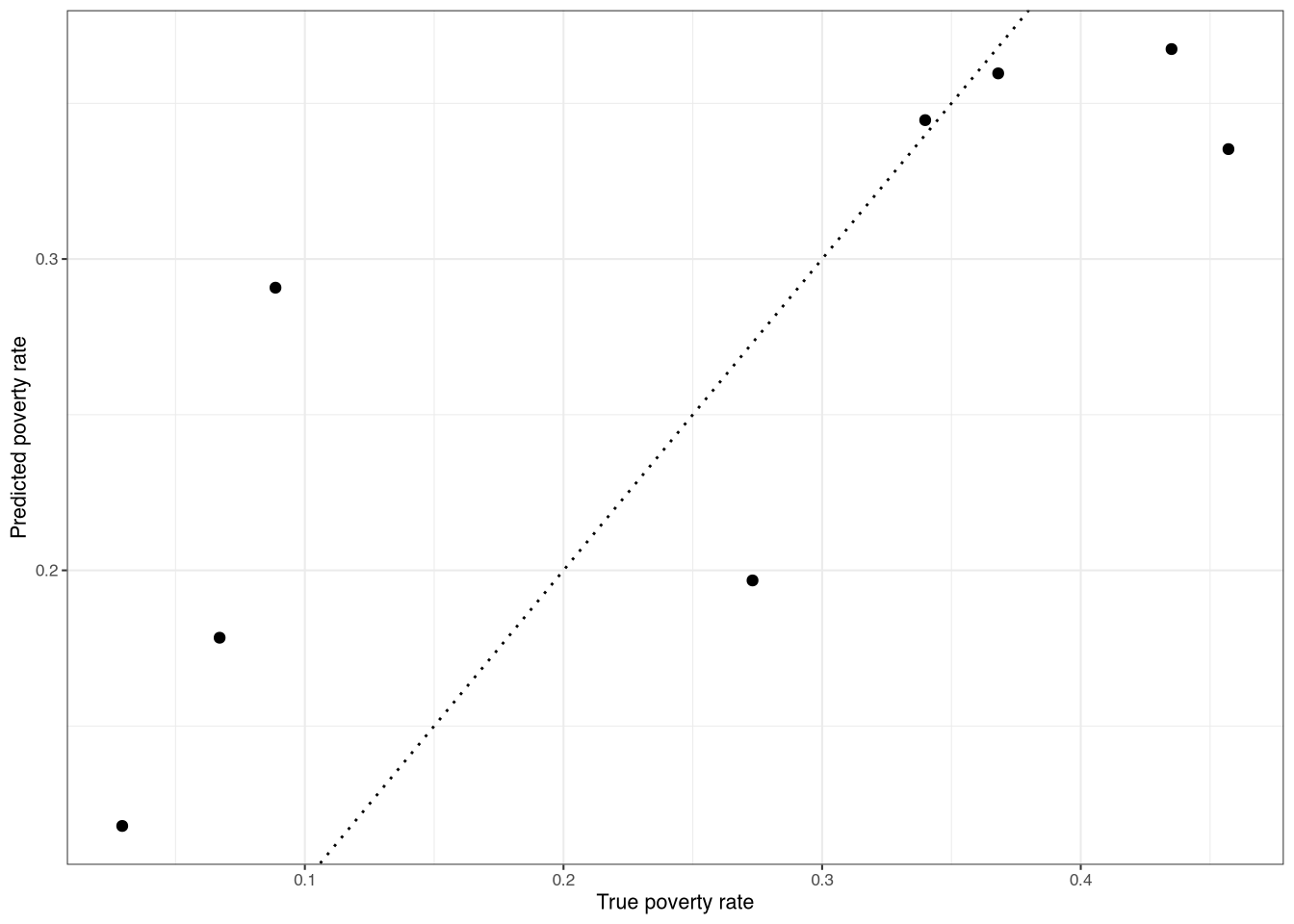
The correlation here is approximately 0.81 for fold one. Note, however, that this could be an underestimate of the true correlation. Why? Because the sample itself has sampling error. This means that the sample estimate is not the “true” value, but rather a (sampled) estimate of it.

7.5 References

Molina, Isabel, and Jon NK Rao. 2010. “Small Area Estimation of Poverty Indicators.” Canadian Journal of Statistics 38 (3): 369–85.

Footnotes

1. It is important to note that are estimate mean squared error (MSE) and not the variance. However, we usually assume they are the same, assuming there is no bias.

2. The plot is not shown here, but you can run it on your own.

3. Note that we create a new weight variable to estimate headcount poverty.